Deionization

Ion Exchange Applications Of Simulation Technology

Ion exchange (IX) continues to gain popularity as the method of choice to removing trace contaminants from potable water, process water, boiler feed waters, and industrial effluents. These are new and rapidly growing applications.

The number of substances listed on the U.S. Environmental Protection Agency’s(EPA) Maximum Contaminants List(MCL) continues to grow. Also, the MCL levels and purity requirements in all applications are becoming more stringent as our ability to measure lower concentrations of all substances and correlate them with health and production, benefits improves. To cite just a few examples, boron, total organic carbon (TOC), arsenic, and perchlorate are now specified to parts-per-billion (ppb) and sodium to parts-per-trillion (ppt) in applications where they were not mentioned 20 years ago.

When trace contaminants are removed, it is not unusual to have two or more trace contaminants being removed simultaneously in a single resin bed. Before simulation technology, there was very little resin performance data available for these kinds of applications. The traditional role of IX resins has been softening and deionization. Performance data for IX resins was developed for predicting capacity and leakage of a single contaminant such as hardness, silica, or sodium. The vast majority of the performance information available today was developed for single ions without regard to how other ions behaved during the service cycle.

In some cases, the service run lengths of the IX resin for trace contaminant removal are enormous compared to softening or deionization. Sometimes it is more practical to change out the exhausted resins for virgin resins instead of regenerating them. In cases where multiple trace contaminants are to be removed by a single resin bed, the potential service cycle for one contaminant will likely be much different than for the other(s). In these cases, the resin is either regenerated, or changed out when leakage of the first contaminant reaches its limiting value.

In softening and deionization applications, 3 to 5 cycles are typically required to reach stability, based on capacity and average leakage of the single controlling substance. In situations involving multiple contaminants of interest, the service cycle has to be limited to the break through of the least preferred contaminant, while also avoiding chromatographic dumping to levels beyond acceptable limits of other substances.

In stable multi-cycle operations, the quantity of each ion absorbed by the resin during the service cycle is equal to the quantity desorbed during the next regeneration. When the regeneration level is set for the contaminant with the lowest affinity, the ions with higher affinities will not be completely removed and will accumulate on the resin. As they accumulate, they become easier to remove and more is removed during subsequent regeneration cycles. This process continues until stability is reached.

The higher the affinity, the more cycles it takes to reach stability for a specific ion. In order to give reliable performance data, a pilot plant study needs to be run until repeat performance from one cycle to the next is achieved for all ions. In order to reach this stability, a pilot plant study must encompass several cycles of exhaustion and regeneration. Just how many cycles depends on the relative affinities of the controlling ions (contaminants).

For example, the relative affinity of calcium to magnesium is about 3 to 1, and it takes about 3 regeneration cycles to reach stable operation in softeners. The relative affinity of perchlorate to nitrate, in a nitrate selective resin is about 100 to 1, and it takes about 100cycles to reach stability. The point here is that the column studies used to make performance estimates for multiple contaminants may need hundreds of exhaustion and regeneration cycles. It could conceivably take several years

to conduct a single column test before reaching stable operation. However, thanks to simulation technology, we can perform simulated pilot plant studies covering hundreds of cycles of exhaustion and regeneration in a few minutes, and provide complete effluent histories for each ion in the liquid and resin phase. Simulation technology can provide additional and new benefits, some of which we will discuss through the following review of a few specific cases. In order to put things into proper perspective, let us review the history of resin ratings, how they were developed, and then applied.

 

History of IX Performance Estimations

The history of IX resin rating programs basically follows this timeline:

• 1930s—IX resin invented
• 1940s—first resin rating available
• 1970s—first resin rating software
• 1980s—software resin ratings widely available
• 1990s—resin rating available online

Catalog and reference libraries of original equipment manufacturers (OEMs), architectural engineers (AEs), consultants, and endusers who design, build, own and operate IX systems, usually include several engineering binders from various resin suppliers. These often contain performance data in graph and table format for various types of resin from which IX resin performance estimate scan be calculated. This information was developed for softening and deionization applications. The information is still considered accurate, and remains widely used, but it was developed for limiting the leakage of a single contaminant, typically those important to boiler feed water requirements.

Examples of rating data can be found in the various resin supplier literature, commonly referred to as engineering bulletins or IX manuals. The performance data shows how much water would passthrough the resin between regenerations at a given regenerant dose and when operated on a specific water composition to a specific leakage endpoint for the key substance.

The various ions in most waters are shown in Tables A through C.

Those ions present in the raw water that were not included in the engineering tables were dealt with by lumping them with ions with similar exchange behaviors. Potassium (K) would be lumped together with sodium (Na), nitrate (NO3) with chlorine (Cl), and carbonate (CO3) with bicarbonate (HCO3), among others.

The early approach using tables and graphs worked well, and effectively handled some complex problems, such as the reaction between hydrogen ions liberated by hydrogen form cation resins with the bicarbonates in the raw water. This reaction reduces the hydrogen ion concentration, which in turn reduces sodium leakage. Silica is poorly ionized in the raw water, but becomes ionized in the high-pH environment of a hydroxide form strongly basic anion resin, and is exchanged onto the resin as the silicate ion.

Although, this type of data could undoubtedly be developed for the newer “emerging” contaminants of interest, the cost can no longer be supported by profit margins on sales of IX resins, nor would such data be available in a timely manner.

The complexities of monitoring and controlling run lengths for more than one trace contaminant, and the multiple possible interactions makes it impractical to conduct real world pilot plant studies, in most cases. The run lengths are usually enormous compared to traditional IX applications. Such a pilot plant study might take years to complete. Due in part to recent software development by one IX resin maker, these kinds of pilot plant studies can now be simulated in a few minutes.

 

Simulation Technology

Before 1980, nitrate was the only anionic contaminant commonly removed by IX for potable water purposes. Other contaminants were present, but typically at such low levels that they were ignored. For example, softeners will remove radium and barium. But, softening is not widely practiced for large potable water treatment systems. In the very late1980s, we started to hear about arsenic. In the 1990s, we became concerned about perchlorate and then more attention focused on radium, barium, selenium and uranium. Trihalomethane (THM) precursors, nitrosamines, ammonia, and phosphate are also receiving attention.

In the last decade, non-regulatory pressure is changing the list of desirable and undesirables. For example, magnesium is gaining attention as a desired substance to keep rather than remove by softening. The magnesium issue is an ongoing effort spearheaded

by recent studies conducted by the WordHealth Organization (WHO). Health food trends are also adding to the list of undesirable substances.

For example, sodium is becoming anon-desirable substance present in softener effluents. In response to this, sales of potassium chloride regenerant salt is growing rapidly as the trend to limit sodium in softened water. There is almost no resin supplier data for regeneration dose of potassium chloride and softener performance or its impact on sodium concentrations in the softened water, which is variable since some waters have appreciable amounts of sodium before they are softened. Fortunately, simulation technology can provide this information on a case-by-case basis rapidly and efficiently to meet the needs of the market for this kind of performance data. The problems of providing performance data for IX resins for these new substances, also to handle the lower levels of the familiar ones are easily and efficiently handled by simulation technology.

Advanced simulation technology combines mass action and kinetic relationships to simulate exhaustion, and regeneration cycles of an IX resin. As of July 2008, one resin maker’s simulation program is designed to deal directly only with ionized substances. The simulation soft water calculates the exhaustion profile for each ion in each portion of the water, and the resin bed as the water (or liquid) passes through the resin. Variations in operating conditions can be studied quickly and efficiently. The program outputs a calculated effluent history for all input ions passing through the resin bed. The results are outputted to a spreadsheet. There is virtually no limit to the number of ions, valences, or number of exhaustion and regeneration cycles that can be studied. The input requirements for a simulation are similar to traditional resin ratings. A full water analyses is required, including concentrations of the ions of interest as well as all the major ions plus effluent goals for each substance of interest, including maximum allowable levels. We have developed the equilibrium and kinetic relationships for a large number of ions. As the need arises, additional ions can be added to the list with relative ease. As an example of the power of simulation software, we have chosen an example of a nitrate removal resin where arsenic, chromium, selenium and uranium are also present. The simulated effluent profile can be used to make informed decisions about where to end the service cycle to avoid chromatographic peaking of trace contaminants. To illustrate the value of IX simulation, we have selected four examples of real world current problems that are not covered by traditional IX resin rating programs, and which cannot be easily predicted by manual calculations. The behavior of many other contaminants can also be modeled by simulation technology of which the possibilities are virtually endless. The contaminants we have chosen for this presentation include:

• Molybdate removal from closed-loop cooling systems.
• Simultaneous removal of per chlorate by regenerable nitrate removal systems.
• Potassium cycle softening.
• Effect of impurity hardness levels in the salt used to regenerate water softeners.

In a more complicated simulation, we looked at water that contained many trace contaminants. First, we ran the simulation well past the complete breakthrough of all anions so we could observe the break through patterns of each ion. We also looked for any chromatographic peaking so we could compare peak and average leakage levels with MCL guide-lines, among others. Then we looked at break through patterns for each ion and for problems like chromatographic peaking. This information is used to determine how best to operate the system. In this case, there is essentially no chromatographic peaking. NO3 and perchlorate (ClO4) levels remain below their MCL limits. Arsenic (As), for a brief period, reaches 6 ppb, then rapidly drops to its influent value of 5.5 ppb. ClO4 begins as low break through at 1,000 bed volumes (BV), and gradually rises to its influent value at around 3,000 BV without noticeable chromatographic peaking. Uranium starts to break through at 50,000 BV, and rises gradually to 90% leakage at 150,000 BV. It was necessary to run two simulations (under 1 minute), one to a much shorter endpoint in order to show the profiles of all species, including those highly preferred.

 

Molybdate Removal

Here is a real world example. In a large office building, the cooling system uses 5,000 gallons of chilled water, contain-ing 200 parts-per-million (ppm) of molybdate, which serves as a corrosion inhibitor. There is no reservoir, the pip-ing system contains the 5,000 gallons. The local ordinance is expected to be changed in the near future, which will prohibit further molybdate use. Access to the system is via a bypass line that can treat only about 10% of the full flow rate while the other 90% passes by.

The enduser wants to explore options as to how best to remove the molybdate replace it with a borate-based inhibitor. At first glance, a portable mixed-bed canister with about 6 cubic feet (ft3) of resin could do the job. But, the pH of the effluent DI water would be below the desired range of 9 to 10. The mixed bed would also remove needed ions to maintain corrosion protection. The operator wants to keep the “non-molybdate” ions intact, and to remove the molybdate to “as close to zero as practical”. Table D provides a water analysis.

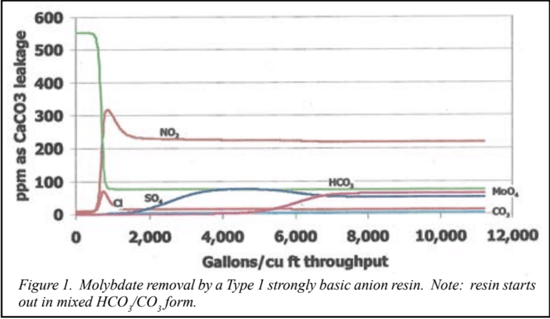
Strongly basic anion-exchange reins are known to have a high affinity for the molybdate anion. However, the selectivity coefficient for molybdate is not readily available from published literature. Our technical support group determined the molybdate selectivity needed to simulate a resin pilot plant based on a Type 1 strongly basic anion resin. We simulated the exhaustion cycle on a full-flow basis to assess the potential least cost (resin wise) approach. We compared this to the simple longer term zero labor approach of simply placing a small portable vessel with a small amount of resin in the bypass line and leaving it operate until it became equilibrated with the 5,000 gallons of the liquid in the piping system.

Figure 1 shows that a single cubic foot (ft3) of resin could handle the job if all the flow could be processed through the resin bed at a reasonable flow rate. It can be seen that about two-thirds of the resin’s capacity is filled by molybdenum before the resin becomes exhausted. However, even if such a scheme could be put into action, it would require full-time monitoring of the influent and effluent to prevent overrunning the bed, or in the case of recirculation, shutting off the flow to the resin bed once the maximum possible reduction of molybdate was accomplished. Otherwise, the molybdate “free” solution would act as a regenerant, and begin pushing molybdate from the resin bed.

The simpler approach was to let the resin bed run under recirculation until the resin and the treated solution were in equilibrium. We simulated the re-circulation of 5,000 gallons of solution through various amounts of resin as a batch treatment system, which showed that a single vessel with less then 2 ft3 of resin left unattended until equilibrated could reduce molybdate to acceptable levels. Continuous recirculation at 4 gallons per minute (gpm) for a month gives more then one full turn over of the system volume per day. Five full turnovers is required at full mixing to reach 99% of equilibrium, but due to the configuration of the system it was felt that the simplest approach would be to replace, or regenerate the resin bed at monthly intervals and monitor results at those times. The simulation using a bicarbonate-form resin showed that the resin loads about 40% of its capacity with molybdenum when operated in this manner. In both cases, the pH remains above 8.9 at all times. We tried different combinations of preloaded ions on the resins and varied the amount of resin. In all, about 15simulated pilot studies were conducted, which required only a few minutes of actual computer time.

 

Simultaneous Nitrate and Perchlorate Removal

The initial simulations show the effluent profiles for the virgin cycle of operation. Two simulations are needed, because perchlorate throughput is so much greater than the other ions.

The existing plant used a “NitrateSelective” resin to prevent the chromatographic dumping of nitrates by sulfates. There were “no perchlorates” in when the plant was built. However, perchlorates are present in the new well. It can be seen that while ClO4 would stay below 4 ppb for more then 20,000 BV, NO3 would exhaust the resin and its leakage would exceed its MCL at about 325 BV. This is a small fraction of the run length to the ClO4 endpoint. The resin is regenerated on NO3 breakthrough. We need to know what will happen to perchlorate leakage over many cycles operated to nitrate breakthrough. To answer this question, we ran a 250-cycle simulation.

The simulated service cycles were terminated and the resin regenerated when nitrate leakage reached 40 ppm. After the first few cycles, perchlorate leak-age appears immediately at ever-higher levels during the exhaustion cycles, and eventually reaches a plateau.

This is not unexpected. Perchlorate is strongly held by the resin. It occupies the portion of the resin bed closest to the inlet.

Nitrate being next strongly held occupies the next level. The regenerant level was selected to maintain low nitrate leakage. Before perchlorate leakage becomes stable, the regenerant must be able to push off as much ClO4 as loaded by the resin during the previous exhaustion cycle. In the early cycles, ClO4 is only partially displaced by the regenerant, and continues to build upon the resin. As the number of cycles increase, the perchlorate zone will be pushed to the exit end of the resin and leakage will appear in succeeding cycles. As the ClO4 continues to build up further, there is more opportunity for it being displaced from the resin bed during the regeneration step. The increased leak-age and build up of ClO4 on the resin from one cycle to the next slows down, until finally as much ClO4 is loaded as is displaced by regeneration, and the operation becomes stable.

The question becomes what, if anything, can be done to reduce perchlorate leakage? One possibility is countercurrent regeneration. IX simulations can be used to predict average leakage of homogenized beds, co-flow, countercurrent, and regenerations at various salt doses, and after stable operation has been achieved. Prior to this work, a small number of laboratory tests had to be performed to develop the chromatographic constants and kinetic factors for the resin. We have developed a database of chromatographic constants for the all of the common ions for several different IX resins as part of the development pro-gram for our simulation technology. We found that small differences in gel-phase composition has a considerable impact on the equilibrium constraints, and also that size distribution affects kinetics. Needless to say, similar products will behave in somewhat similar fashion, depending on how similar they are. What about using higher salt regenerant dosages? Figure 2 shows the effect of using a single massive regenerant about 50 times the normal dose level. It shows leakage was reduced, but only by about 20%.

 

Potassium Form Softening

Potassium cycle softening is an excellent way of maintaining low-sodium effluents from a water softener. Simulations can be used to generate capacity and leakage curves that are similar to traditional resin ratings. However, traditional softening data has little to offer regarding sodium leakage, or operating capacity versus dose in potassium cycle softening. This is a case where two sets of ions are controlling hardness and sodium. Figure 3 shows the sodium leakage from a softener operating in the potassium cycle (regenerated with potassium chloride [KCl]). It can be seen that there are two parts of the service cycle, low Na, and relatively higher sodium leakage. In the early part of the service cycle, sodium from the raw water is removed along with the hardness by exchange for the potassium on the resin. As the service cycle progresses, calcium and magnesium occupy the inlet portion of the resin, pushing the sodium the towards the exit end of the resin bed. Once all the potassium is consumed, the softener will continue to function as a softener by operating in the sodium cycle by discharging the previously loaded sodium from the raw water until hardness break. A simulation shows how much of the run is truly low sodium water and the operating capacity to the end of the low sodium portion of the service cycle, the end of the softening cycle and the sodium levels for either portion or both combined. This information is useful for determining the optimum point to terminate the exhaustion cycle.

 

Softening Problems

Design data for softeners were published with assumed salt purity levels. In the real world, salt purity varies widely.Leakage information, based on the level of salt purity was then used as the platform to make predictions at other operating conditions including variations in TDS.

Figure 4 shows the run length and leakages for a standard water softening resin operated at various regenerant levels of a chemically pure salt regenerant. The capacities are quite similar to those found in design engineering notes provided by resin suppliers, except for the leakage values.

Leakages shown in the simulation, while similar, are a bit lower, because the simulation was run with a regenerant brine with zero hardness. Hardness leakages are determined, to some extent, by the salt purity and usually to a larger extent, the dose level, raw water total dissolved solids (TDS), and the regenerant process itself, countercurrent or cocurrent regeneration. The regenerant brine concentration is also an important factor, especially in critical applications. Regenerant contact time affects capacity and leakages in opposite ways. The resin supplier engineering notes are of necessity simplifications of several factors to make a standard case. The next few figures will show what happens when some conditions held constant inthe engineering bulletins are varied.

Figure 5 compares cocurrent and countercurrent regeneration in a water stream with relatively low TDS (same regeneration dose) using pure NaCl as the regenerant against the lower purity rock salt. Note that for low-TDS waters such as this, there is not a lot of difference in leakage when using chemically pure salt or rock salt.

In Figure 6, the same comparison is made, but the water contains more hard-ness, and a higher TDS.

At higher TDS, the effect of hardness in the salt is magnified, particularly with coflow regeneration. In a well-operated countercurrent regenerated system, the hardness leakage is almost entirely dependent on the salt purity (hardness impurity). In cocurrent regeneration, all the hardness in the exhausted resin is pushed through the exit end. So in a cocurrent regenerated system, the exit end of the resin bed sees spent brine with hardness mixture as the regenerant.

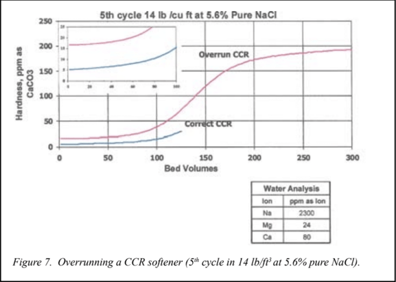
In well-operated countercurrent regenerated systems, the resin beds are not allowed to fully exhaust. When the service cycle is terminated, there is a substantial amount of sodium left on the resin at the exit end of the resin.In the countercurrent regeneration, the regenerant inlet is the same end as the service cycle exit. So, the purest form of the regenerant solution contacts this end first. Therefore, the composition of the exit end of the resin bed in the service cycle is determined by the purity of the salt and the TDS level for a given hardness endpoint. The hardness endpoint can be as important as the salt purity in determining the hardness leakage in subsequent service cycles. This slide shows the impact of over running the resin bed, or running the service cycle to a higher hardness leakage endpoint on leakage quality.

Figure 7 would be identical to Figure 6 except for a 15% difference in run length. Shortening the run length by15% reduced leakage in the countercurrent regenerated to one third. The same change in the cocurrent regenerated resin bed had only a 20% impact on leakage. It is well known that overrunning a countercurrent regenerated resin bed has a very negative impact on leakage quality. There is no engineering data for this effect, because of the complex interaction of all the different variables. This makes it almost mandatory to run a pilot plant for each case to be studied.Simulation technology lets us do this quickly and efficiently. These slides also show how important salt quality is when using countercurrent regeneration to produce low-hardness effluents.

 

Closure

Simulation technology can replace physical pilot plant studies providing data in minutes that might otherwise take years. It can simulate cocurrent, countercurrent, and homogenized bed regeneration techniques for as many cycles as desired. It can show chromatographic peaking for multiple ions simultaneously. It can predict complex changes in operating systems when inlet water compositions change, such as in switching supply sources on operating systems. Models of IX systems can be used as a tool in the process design of an IX system and as a troubleshooting tool to examine behavior of systems already in operation.

Bibliography

Anderson, R.E. “Estimation of Ion Ex-change Process Limits by SelectivityCalculations”, AIChE Symposium Series, 7l, p. 152, 236 (1975).
Clifford, D. “MuIti-Component Ion-Exchange Calculations for Selected Ion Separations”, Industrial Engineering Fundamentals 21(2), p. 141 (1982).
Crits, G.J.; Valentine, D.H. “The Significance and Limitations of Laboratory Resin Analyses in Evaluating Ion Exchange Operating Performance”, International Water Conference, Pittsburgh, Pa. (Oct.24-26, 1988).
DeSilva, F.; Gottlieb, M. “A Software Model for Optimizing Resin Selection”, 28th Liberty Bell Corrosion Course (September1990).
DeSilva, F.; Gottlieb, M. “The Relationship between Resin Operating Capacity and Static Analysis Results”, Proceedings of ULTRAPURE WATER Expo East, Philadelphia, Pa. (April 29 - May 1, 1991).
Gottlieb, M. “Economic Considerations in the Selection of Ion Exchange Resins”, 24th Liberty Bell Corrosion Course, Philadelphia, Pa. (September 1986).
Gottlieb, M. “Performance Projections for Anion Resins in Two-Bed Demineralizers”, International Water Conference, Pittsburgh, Pa. (Oct. 23-25, 1989).
Gottlieb, M.; DeSilva, F. “Economic Considerations in the Replacement of Ion Exchange Resins”, I.S.P.E. EXPO ’92, Philadelphia, Pa. (May 7, 1992).
Guter, G. “Nitrate Removal from Contaminated Water Supplies’, Vol. ll, EPA Report, U.S. Environmental Protection Agency, EPA/600IS2-871034 (August 1981).
Guter, G. “Estimation of Effects of Resin and Water Composition on Column Performance in Nitrate Ion Exchange”, American Water Works Association Conference, Dallas, Texas (June 10-14, 1984).
Guter, G. “Removal of Nitrates from Contaminated Water Supplies Using Tributylamine Strong Base Anion ExchangeResin”, U.S. Patent 4,479S77 (Oct. 30, 1984.)
Guter, G.; Hardan, D.L. “Computer Simulations of Nitrate Removal by Ion Exchange”, Proceedings of the AWWA 1985 Annual Conference Proceedings, Washington,D.C. (June 23-27 1985).
Guter, G.; Hardan, D. “Computer Simulation of Nitrate Removal by Ion Exchange”, Boyle Engineering Corp., Bakersfield,Calif. (1985).
Guter G.; Rowles, R.; Kartinen, E. “TheEconomics of Nitrate Removal in the Los Angeles Basin: A Case History”, Boyle Engineering Corp., Bakersfield, Calif.(1985).
Guter, G. “Nitrate Removal from Contaminated Water Supplies”, U.S. EnvironmentalProtection Agency Project Summary,R&D EPA/600/S2-87/034, Vol. 2 (August 1987).
Guter, G. “Reclamation of Waste Brine fromNitrate Removal Plants”, Report, Guter,County of Kern, Calif., Community Devel-opment Department (October 1990).
Guter, G.; Rowles, R.L.; Kaninen, E. "Economics of Nitrate Removal in the Los Angeles Basin, A Case History”, 1991 American Water Works Association Annual Conference, Philadelphia, Pa. (June23-27, 1991).
Guter, G. “Removal of Nitrate from Contaminated Water Supplies for Public Use:Final Report”, U.S. Environmental Protection Agency, EPAdoOlS2-82-a42 (August.1992).
Helfferich, F. Ion Exchange, McGraw-HillBook Co, New York, N.Y. (1962).
Helfferich, F.; Klein, G. Multi-Component Chromatography Theory of Interference, Marcel Dekker Inc., New York, N.Y.(1970).
Kunin, R. Ion Exchange Resins, Robert E.Krieger Publishing Co., Malabar, Fla., p.16 (1958).
Liang, S.; Guter, G. “Nitrate Removal from Contaminated Groundwater”, Journal of the American Water Works Association 91(2)(February 1999).
“Nitrate Removal from Contaminated Groundwater by Anion Exchange”, Chapter 2 inIon Exchange Technology Advances in Pollution Control, SenGupta, A.K., ed., Technomic Publishing, Lancaster; Pa.(1995).
Simon, G.P. Ion Exchange Design Manual, Reinhold Publishing Corp., New York, N.Y.(1991).